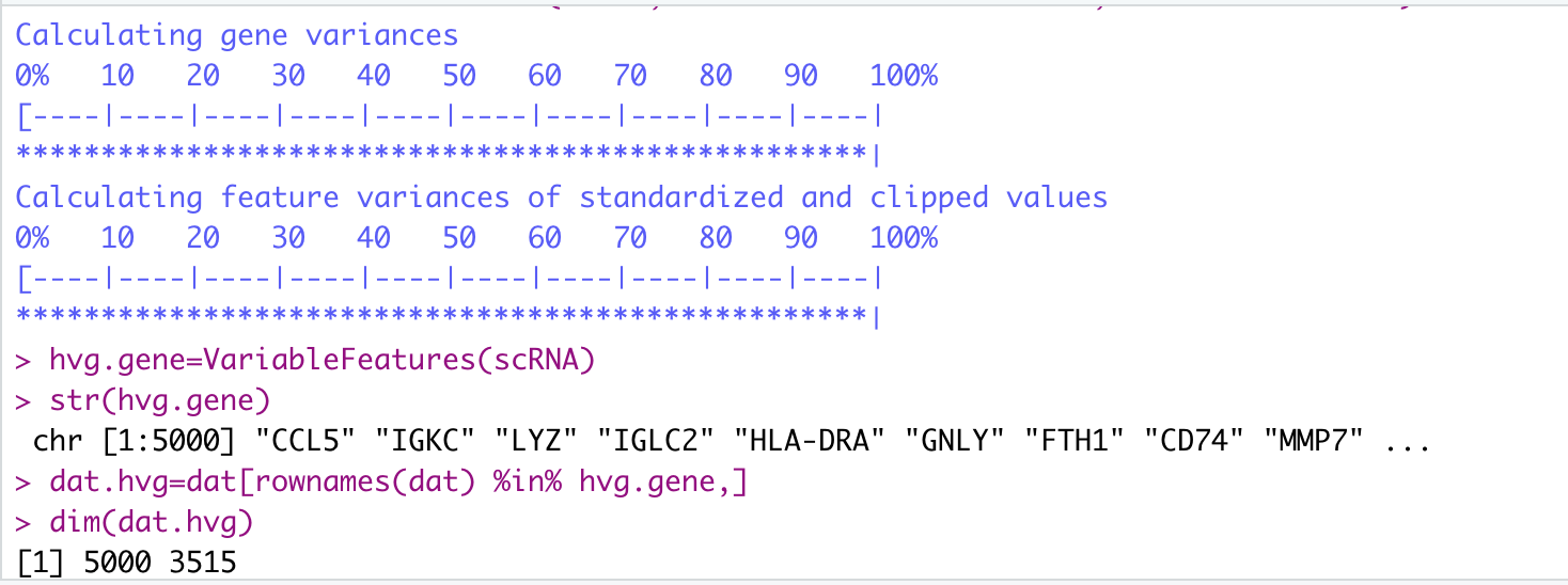
Recover one figure from public paper.
Material and methods
-
Data set:
GSE122083/GSM3454528 -
R package:
Seuratandigraph
Step 1. QC
-
Download data
-
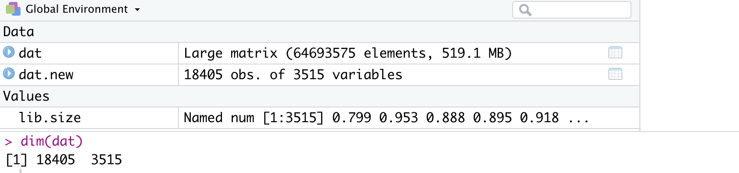
Load data
-
Remove duplicated genes and Select max expression
|
|
- Normalizing the data
|
|
- Transform with log2()
|
|
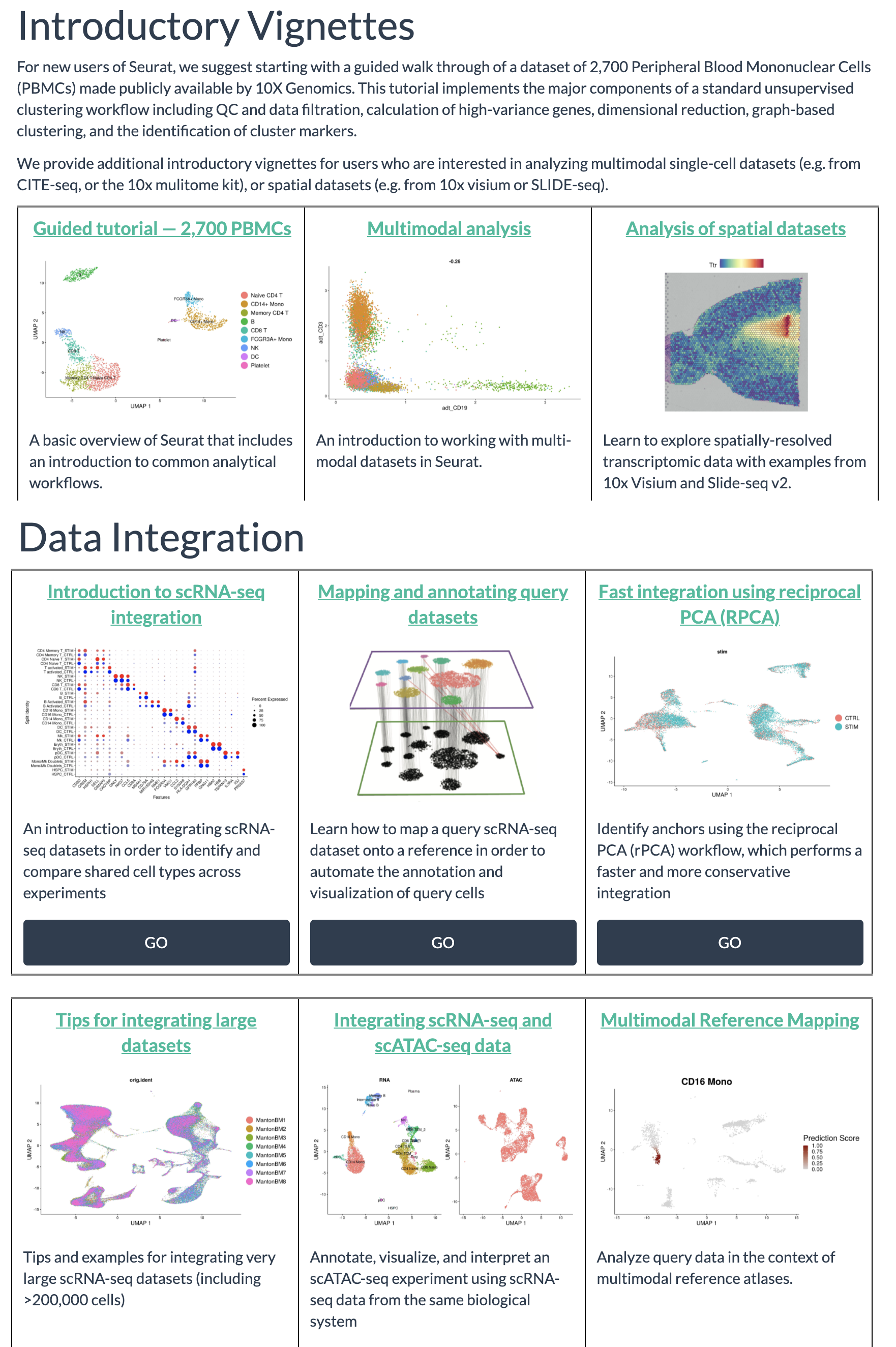
Step 2. Identification of highly variable features (top5000 genes) for PCA analysis with Seurat package
-
Seurat is a toolkit for quality control, analysis, and exploration of single cell RNA sequencing data.
-
Setup the Seurat Object
|
|
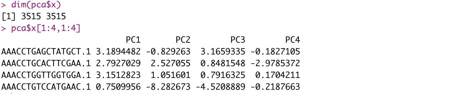
- PCA with
prcomp()
|
|
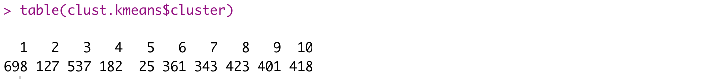
Step 3. k-means cluster
|
|
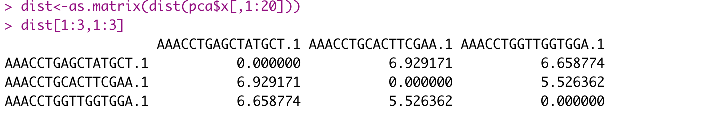
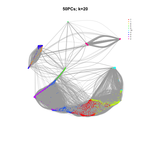
Step 4. KNN visualized
|
|
|
|
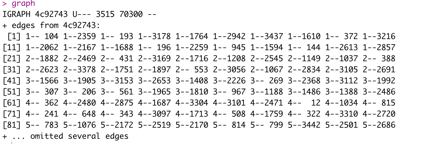
- Create igraph
|
|
|
|
- Define function(D,k) to enable to try different k
|
|
- Plot with different k values
|
|
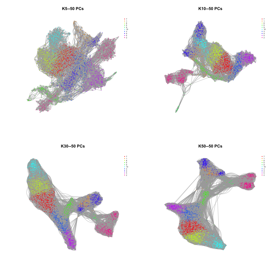
In summary
-
PCA and KNN are common methods, herein, they are standard ways to implement.
-
Keep different parameters could get different results.